Real Estate Financial Modeling (REFM): The Ultimate Guide, With Templates & Examples

When it comes to real estate financial modeling (REFM), there’s a ton of information out there…

…which, ironically, makes it harder to understand.

It can be nearly impossible to find one source that clearly explains the key points from start to finish.

We go into great depth in our full Real Estate Financial Modeling course, so I’m not going to attempt to replicate everything here.

However, I will summarize the most important parts, give you a few sample Excel (XLS) models to download, and explain the step-by-step process for modeling the three most common deal types:

• Acquisition
• Renovation
• Development

So let’s get started…

Real Estate Financial Modeling: Sample Excel (XLS) Files

Here are the sample Excel files (both simplified real estate models). Below, we’ll move on to the explanation and tutorials.

• Multifamily Acquisition Model – Arcadia Gardens (XLSX)
• Industrial Development Model – 4216 61 Ave SE (XLSX)

What’s the Point of Real Estate Financial Modeling?

First, some definitions: we define “real estate” as land and buildings that generate revenue or have the potential to do so.

We focus on commercial real estate (CRE) that is purchased and then rented out to individuals or businesses, as opposed to residential real estate, such as single-family homes, that is owner-occupied and not rented out to others.

In CRE, individuals or businesses, i.e., tenants, pay rent to property owners to use their space.

The owners earn income from this rent, and they use part of it to pay for expenses such as utilities, property taxes, and insurance; in some cases, tenants are responsible for portions of these expenses as well.

All of this allows us to come up with the following definition of Real Estate Financial Modeling (aka REFM):

In real estate financial modeling (REFM), you analyze a property from the perspective of an Equity Investor (owner) or Debt Investor (lender) in the property and determine whether or not the Equity or Debt Investor should invest, based on the risks and potential returns.

For example, if you acquire a “multifamily” property (i.e., an apartment building) for $50 million and hold it for 5 years, could you earn a 12% annualized return on your investment?

Or, if you develop a new office building by spending $100 million on the land and construction, and then you find tenants, lease out the property, and sell it, could you earn a 20% annualized return?

If you identify the most important assumptions and set up your analysis correctly, real estate financial modeling helps you answer these types of questions.

All investing is probabilistic, so a simple model cannot tell you if a property will generate an 11.2% or 13.5% annualized return.

But a decent analysis can tell you whether or not that range of returns – 10% to 15% – is plausible.

These are the questions that real estate private equity firms think about all day, and they spend significant time doing the analysis before making investment decisions.

Types of Real Estate Financial Modeling

Real estate combines elements of equities and fixed income and can offer a risk / potential return profile that is somewhere in between them.

For example, a Core real estate deal where a firm acquires a stabilized property, changes very little, and then re-sells it, might offer risk and potential returns closer to those of an investment-grade corporate bond.

On the other hand, a “Value-Added” deal where a firm acquires a property with a low occupancy rate, make significant renovations to improve it, and aims to sell the property for a significantly higher price might offer risk and potential returns closer to those of stocks.

And an “Opportunistic” deal where a firm develops a new property from the ground up (“development”) or completely converts or re-builds an existing one (“redevelopment”) might offer even higher risk than stocks, but also higher potential returns.

These descriptions highlight the three main strategies and the three main types of real estate financial modeling:

• Real Estate Acquisition Modeling: Acquire an Existing Property, Change Little to Nothing, and Sell It.
• Real Estate Renovation Modeling: Acquire an Existing Property, Change It Significantly, and Sell It.
• Real Estate Development Modeling: Buy Land, Pay to Build a New Property, Find Tenants, and Sell It Upon Stabilization.

There is a fourth strategy as well: develop a new property, but pre-sell units before completion rather than leasing it out and selling the entire property at the end.

This type is just a subset of real estate development modeling, and it mostly applies to condominiums (residential real estate), so it’s not our focus.

In addition to these strategies, there are also different property types:

The lease types explain the key differences here.

Office, retail, and industrial properties tend to use more granular financial modeling because lease terms vary significantly, and there are fewer tenants or guests than in multifamily or hotel properties.

By contrast, hotels use assumptions and drivers that you’d see for many normal companies, and multifamily properties (apartment buildings) are somewhere in between.

You can think of the property spectrum like this:

For more about individual properties and how the differences translate into revenue and expenses, please see our detailed article on the real estate pro-forma.

The Step-by-Step Process to Real Estate Financial Modeling

The exact steps vary based on the type of financial model, but they’ll always be something like this:

• Step 1: Set up the Transaction Assumptions, including those for the size of the property, the purchase price or development costs, and the exit (i.e., how much you might sell the property for at the end).
• Step 2: For a development model, project the Construction Period, usually on a monthly basis, and draw on Debt and Equity over time – not all upfront – to fund the construction.
• Step 3: Build the Operating Assumptions for the property, which could be very high-level (e.g., Average Rent per Unit * # Units) or very granular (revenue, expenses, and concessions for individual tenants) depending on the property type.
• Step 4: Build the Pro-Forma, including revenue and expenses down to the Net Operating Income (NOI) line, capital costs below that to calculate Adjusted NOI, and Debt Service (interest and principal repayments) below that to calculate Cash Flows to Equity.
• Step 5: Make the Returns Calculations, including the initial investment and any additional investments over time, the Cash Flows to Equity each year, and the exit proceeds, including repayment of Debt and transaction fees. You focus on the Internal Rate of Return (IRR) and Cash-on-Cash or Money-on-Money multiples here.
• Step 6: Make an Investment Decision based on your criteria and the output of the model in different cases.

Deal Type #1: Real Estate Acquisition Modeling

Let’s begin by looking at a very simple example of a real estate acquisition model for a multifamily property in Arizona. You can download the Excel file here:

• Multifamily Acquisition Model – Arcadia Gardens (XLSX)

This is a 76-unit property that we plan to acquire for just under $10 million USD.

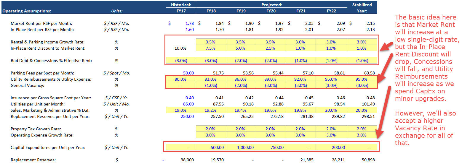
We will change it a little bit because we plan to boost rents up to market rates by lightly renovating the units.

You can determine what these “market rates” might be with some commercial real estate market analysis.

We will also be less generous with concessions, bargain for higher utility expense reimbursements, and accept a higher vacancy rate in exchange for those.

These changes are minor compared with a true renovation or redevelopment, so this deal falls under the “Core” or “Core-Plus” category.

NOTE: In all the screenshots below, you can always click the screenshot to view a larger, higher-resolution version.

Step 1: Set Up the Transaction Assumptions

First, we need to determine the size of the property, which is usually based on the Units times the Average Square Feet per Unit in the multifamily sector:

A portion of the building will not be rentable because it corresponds to hallways, elevators, lobbies, etc., so we also distinguish between gross and rentable square feet:

We then make assumptions for the Acquisition Price, Exit Price, and the Loan-to-Value (LTV) Ratio:

We’ve hard-coded the acquisition price here, but it’s based on a Cap Rate of 5.80%.

That means that we take the Year 1 Net Operating Income (NOI) of the property ($567K) and divide by the 5.80% to determine the price.

NOI is a bit like EBITDA for normal companies: it includes operating revenue and expenses, but not Debt Service – and it may include the capital cost reserves as well, which makes it different from EBITDA.

In real estate financial modeling, property valuation is almost always based on the NOI divided by a Cap Rate or range of Cap Rates.

Cap Rates represent the property’s location, quality, and overall desirability, and lower Cap Rates mean the property is more expensive, while higher Cap Rates mean the opposite.

A multifamily property in Manhattan might sell for a Cap Rate of 3-4%, while a similar one in Columbus, Ohio might sell for a Cap Rate in the 6-8% range.

If the property does not change significantly, it’s best to make a conservative assumption that the Cap Rates rise over time.

We assume here that the Cap Rate rises from 5.80% upon purchase to 6.00% upon exit.

The LTV is 65%, which means that ~$6.4 million of this ~$9.8 million purchase price will be funded with a Senior Loan.

This amount of leverage is very high, but it’s common for properties because:

• Property margins tend to be much higher than “normal company” margins, which gives properties more cash flow to service their Debt.
• Permanent real estate loans tend to amortize over long periods, such as 30 years, which means only ~3.3% of the principal must be repaid each year. Interest-only periods, in the beginning, are common as well.

Using these assumptions, we create a Sources & Uses schedule that shows where the money is coming from and where it’s going to:

Step 2: Project the Construction Period

This step is not applicable here since there is no construction.

Step 3: Build the Operating Assumptions

The key assumptions for a multifamily property include the rent per unit or rent per square foot, the parking income, the utility reimbursements and concessions, and the expenses: insurance, utilities, sales & marketing, property taxes, maintenance, and other operating costs.

The growth rates for all of those, especially the income sources, are also important.

For more, please see the real estate pro-forma for full explanations of these categories:

We use a simple approach here and make the rent and expenses grow at specific annual rates.

Some items are projected on a per-unit or per-square-foot basis, while others are linked to Effective Gross Income (EGI), which is similar to Revenue.

Step 4: Build the Pro-Forma

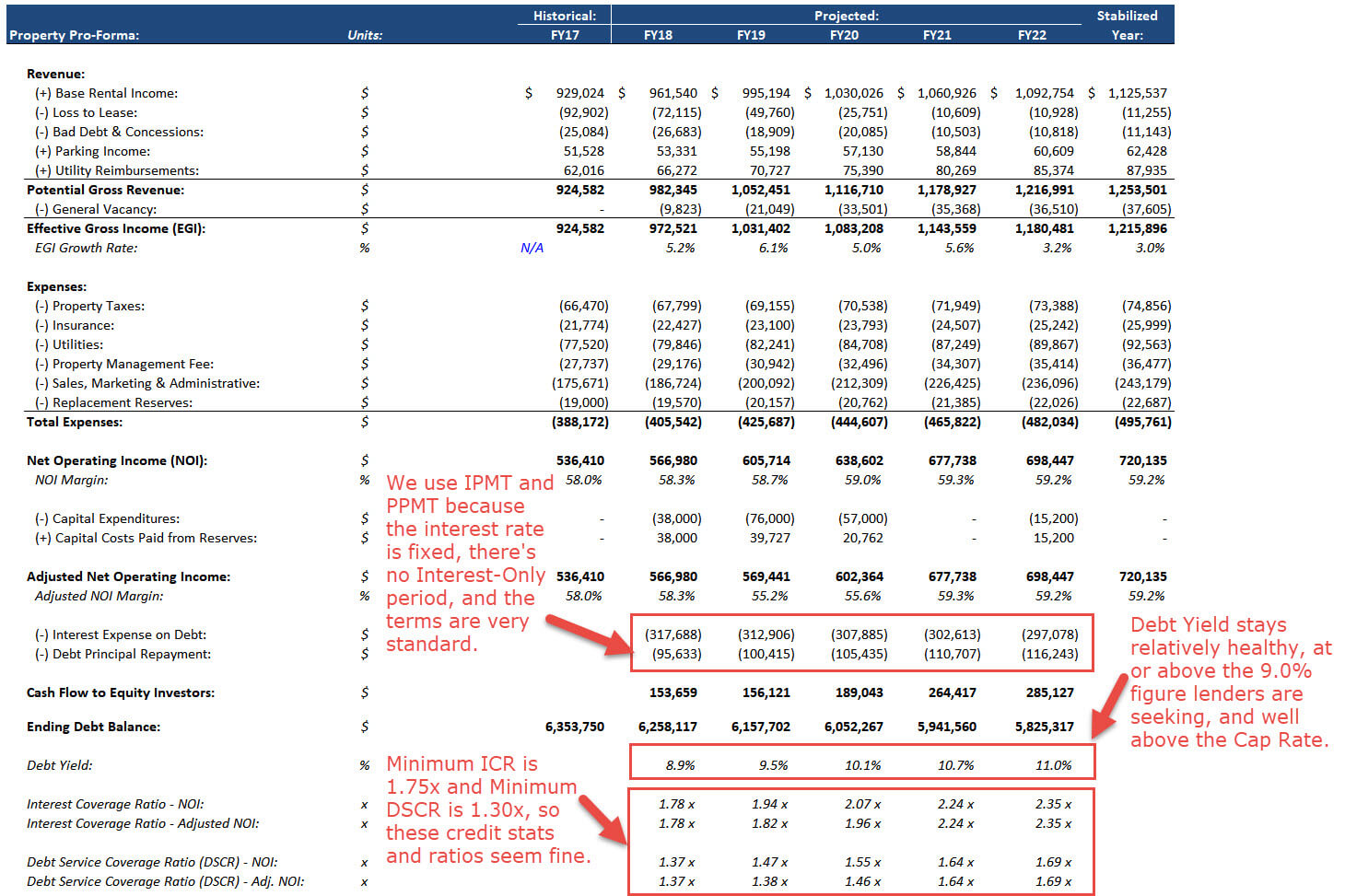
With all these assumptions, we can create the real estate pro-forma:

We use the IPMT and PPMT Excel functions to calculate the Interest Expense and Principal Repayments:

• =IPMT(Loan Interest Rate, Year #, Loan Amortization Period, Loan Amount)
• =PPMT(Loan Interest Rate, Year #, Loan Amortization Period, Loan Amount)

Using these functions ensures that the total amount of Debt Service will be the same each year.

That’s fine here because the terms of the Debt are simple: there’s a fixed annual interest rate, fixed amortization period, no accrued interest, and no interest-only period.

The Debt Yield equals NOI / Initial Debt Amount, the Interest Coverage Ratio equals NOI / Interest, and the Debt Service Coverage Ratio equals NOI / (Interest + Principal Repayments).

In real estate financial modeling, these metrics are important for both lenders (they indicate downside risk) and owners (they indicate Debt capacity).

Step 5: Make the Returns Calculations

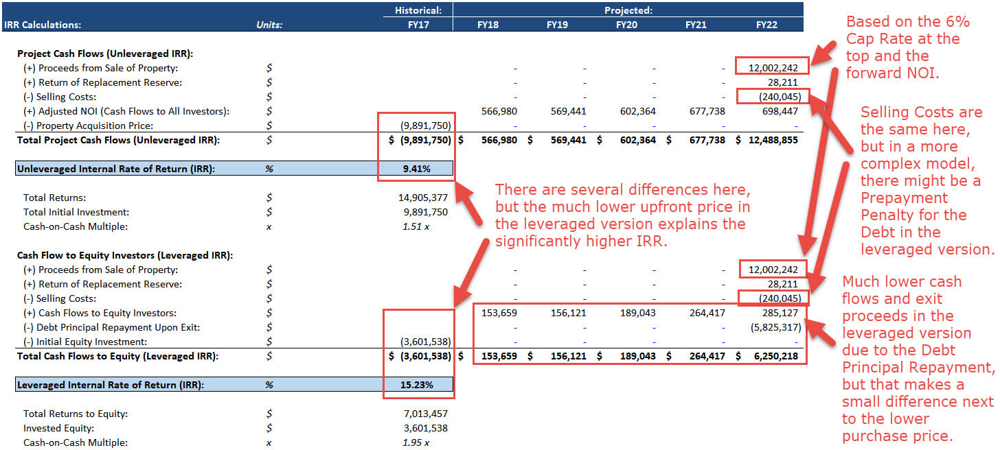
The calculations are straightforward when there’s a fixed exit date in Year 5.

We calculate the returns on an unleveraged basis (as if no Debt were used, meaning no Debt Service and no principal repayment at the end, but a higher upfront purchase price) and a leveraged basis (the traditional method):

We calculate both types of returns to assess how dependent the deal is on leverage.

High dependency could be a red flag since leverage also hurts us if the deal goes poorly.

Step 6: Make an Investment Decision

As always, the answer depends on the IRR our firm is targeting.

For “Core” deals, an Equity IRR of 8-10% is often the target, so by that metric, this deal is a clear “Yes.”

However, to answer this question in real life, we’d have to build sensitivity tables or scenarios and examine other outcomes.

If the IRR drops to 0% with slightly more negative assumptions, then it might be a “No” decision since that indicates too much risk.

It’s also worth evaluating the operating assumptions to see whether or not they’re plausible – if not, then this could also be a “No” decision.

The Cap Rate assumptions seem OK since the Exit Cap Rate rises slightly, and the NOI increases at an annualized rate of around 5%, which is not crazy for a stabilized property.

One potential red flag, though, is that there are no assumptions for Leasing Commissions (LCs) or Tenant Improvements (TIs), even though there will be significant tenant turnover.

Multifamily properties tend to have low LCs and TIs because individual tenants have little bargaining power, but there’s usually at least something in these categories.

Deal Type #2: Real Estate Renovation Modeling

Real Estate Renovation Modeling is quite similar to Acquisition Modeling, and the basic steps in the process are the same.

The key difference is that something significant about the property changes during the holding period, and the owners spend something to enact this change.

For example, maybe they complete a major renovation that boosts a property from Class B to Class A, or they boost the Occupancy Rate from 70% to 90%, or they modify the ground floor of an office building and add retail units.

These differences translate into the following real estate financial modeling additions:

1. Renovation Costs – These will reduce Cash Flow to Equity; you might also assume a higher upfront purchase price to cover these costs, depending on the timing.
2. Penalty During the Renovation Period – For example, a hotel’s occupancy rate might drop as rooms become unavailable due to the renovation.
3. Benefit Following the Renovation – For example, the occupancy rate or average rent might increase once the renovation is done.
4. Permanent Loan Refinancing – There is often a loan refinancing as the renovation finishes and the property stabilizes, both to boost returns for the Equity Investors and to bring in a different set of lenders.
5. Exit Assumptions – It is reasonable to assume a lower Cap Rate upon exit because the property should become more valuable as a result of the renovation.

We’re not going to cover a full renovation example because it’s not much different from acquisition modeling, and this article is already very long.

However, you can get a sense of how the cash flows differ by reviewing the Returns Calculations in a hotel renovation deal:

You can also see why the owners choose to refinance here: doing so at a higher LTV, based on higher NOI, generates around $50 million of Cash Flow to Equity in Year 2, boosting the IRR and Cash-on-Cash Multiple.

Deal Type #3: Real Estate Development Modeling

Real estate Development Modeling could be described as “startup meets leveraged buyout.”

It’s a bit like modeling a tech or biotech startup because you assume an asset gets created from the ground up, but you use both Debt and Equity to fund it – similar to a leveraged buyout.

That setup works because Equity must be contributed first.

Lenders will only sign onto deals once the investors/owners/developers have contributed sufficient Equity to pay for the initial costs – similar to how venture lenders operate.

The last steps in a real estate development model, such as the operating assumptions, pro-forma, and returns calculations, are similar to the ones in the acquisition model above.

The major differences occur in the first few steps because the “purchase price” is based on land and construction costs (not Cap Rates and NOI), Debt and Equity are drawn on over time (not all upfront), and the construction could take years to complete.

We’ll look at a simplified industrial development model here for a plot of land in Alberta, Canada:

• Industrial Development Model – 4216 61 Ave SE (XLSX)

We plan to purchase 18 acres of land, build a warehouse-like facility, and lease it out to two major tenants.

It will cost $12.6 million for the land, $16.9 million for the construction, and $600K for the Replacement Reserves just before tenant move-in, for a total of ~$30 million.

Once the tenants have moved in and the property has stabilized, we’ll sell the excess land and eventually sell the property itself.

Step 1: Set Up the Transaction Assumptions

First, we make assumptions about the construction start date, the plot of land, and the construction costs per gross square foot or gross square meter:

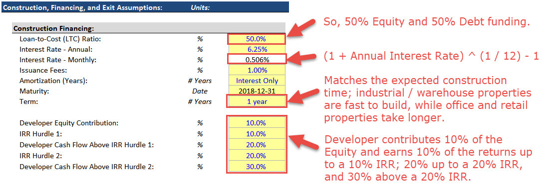
Next, we assume that a Construction Loan is used to fund part of the development costs.

As discussed in our coverage of commercial real estate lending, Construction Loans have higher interest rates than Permanent Loans, and interest is capitalized when the property is under construction:

The IRR hurdles here create a “waterfall model” because the deal’s overall performance changes the percentage that goes to the Developers vs. Investors.

In real estate development deals like this one, Developers often earn higher percentages when the deal’s IRR increases; the waterfall structure incentivizes them to perform well.

Finally, we set up a Sources & Uses schedule:

Step 2: Project the Construction Period

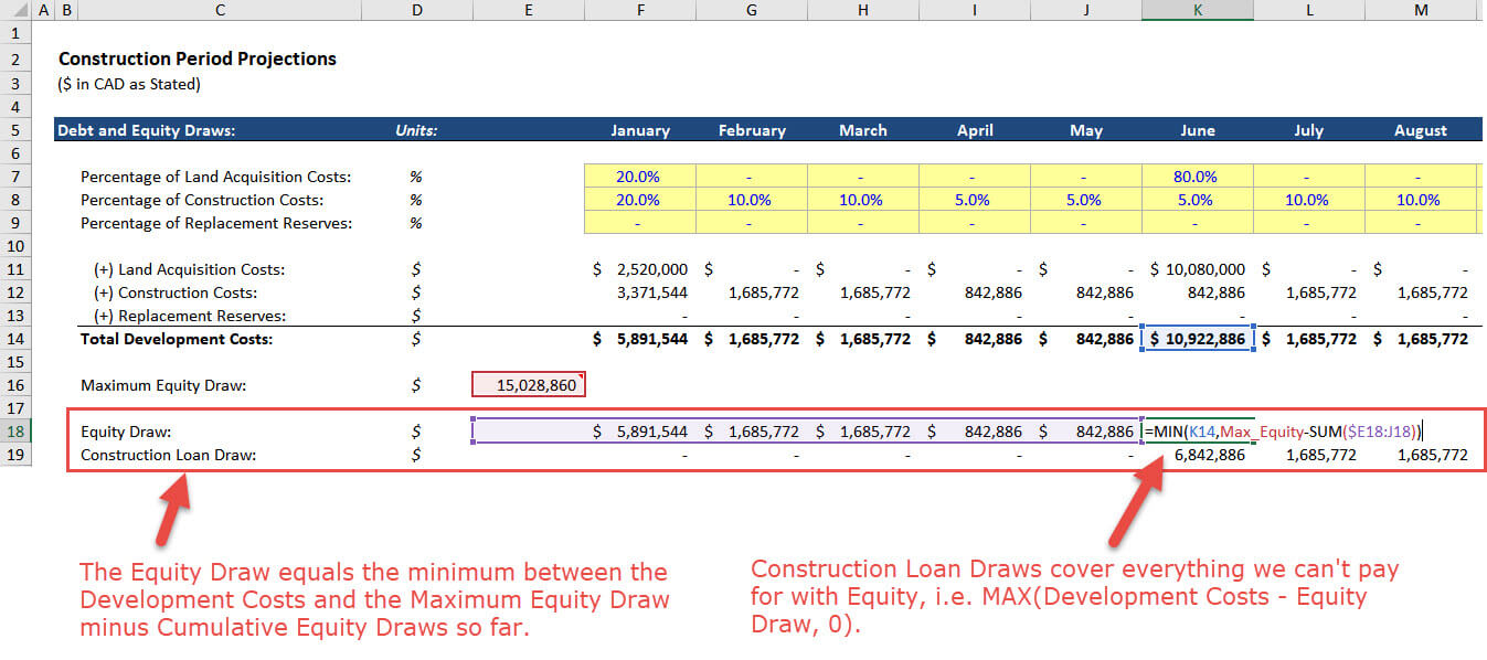
In the next step, we project the Construction Costs over the year required to build this warehouse (the cost distributions here come from an “instructions” document):

Initially, we draw on Equity to pay for the construction, but we switch to the Construction Loan once the maximum amount of Equity has been drawn ($15 million, roughly half the total costs):

The Debt balance must include both capitalized interest and capitalized loan fees – but we base the interest on the beginning balance each month to avoid circular references.

After setting this up, we extend these projections until the end of the Construction Period to get the ending Debt and Equity balances.

They do not represent an exact 50/50 split due to the capitalized loan fees and interest.

In more complex real estate financial modeling exercises, we fix this issue by making the entire calculation circular, but it’s not worth the time/hassle/headache in a quick model like this one.

Step 3: Build the Operating Assumptions

The tenant-by-tenant projections are similar to the setup in the real estate pro-forma article: we assume a rent-per-square-foot figure for each tenant, an annual growth rate, and we use that to calculate the Base Rental Income.

Then, we calculate the Absorption & Turnover Vacancy in periods when tenants might cancel and leave space vacant, calculate Free Rent when new tenants move in, and factor in Expense Reimbursements.

We also calculate the TIs and LCs for each tenant based on the lease start dates and renewal dates.

Step 4: Build the Pro-Forma

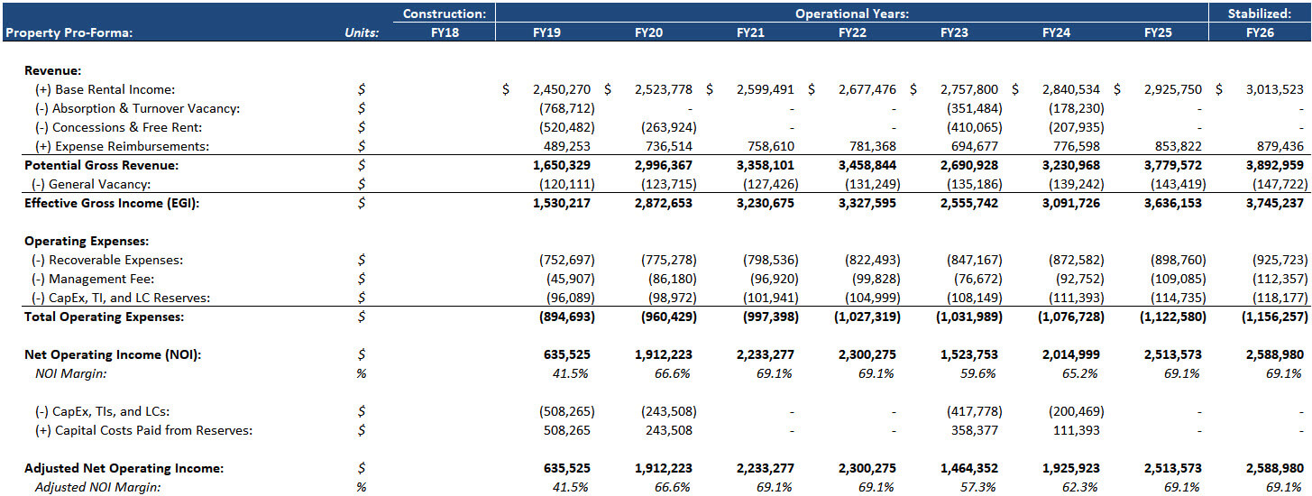
With the tenant assumptions in place, we create the pro-forma:

The Debt Service is a bit trickier because we assume that the Construction Loan is refinanced with a Permanent Loan.

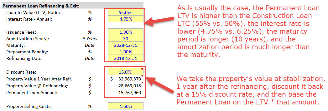
To determine the Permanent Loan amount, we need to estimate the property’s value when the refinancing takes place and then multiply its value by an LTV.

But the property is not yet stabilized when the refinancing takes places, so we retrieve its value one year after the refinancing and discount it back one year:

Next, we project the interest and principal repayments for this Permanent Loan.

There is only one tranche of Debt here, the interest rate is fixed, there’s no interest-only period, and there’s no capitalized interest, so we use the built-in IPMT and PPMT functions in Excel:

Step 5: Make the Returns Calculations

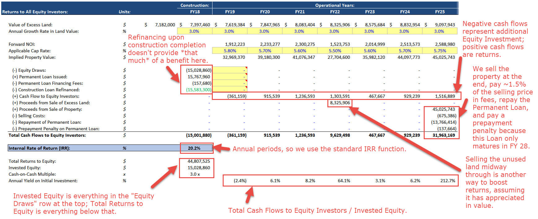
We can now calculate the IRR to Equity Investors based on their initial contributions, the refinancing, the annual cash flows, and the eventual sale of the property.

We’ll also factor in the fees associated with the refinancing, the sale of excess land, the costs associated with the sale of the property, the repayment of Debt upon exit, and prepayment penalties associated with that.

Here’s the calculation with an assumed exit in the final year:

We are simplifying this setup by pretending that the Equity Draws occur all at the end of the first year, not over the first several months of that year.

Also, this model does not support variable exit dates.

Past this point, we create a waterfall schedule to split up the cash flows to the Developers and Investors based on the overall Equity IRR.

We’re not going to cover that here, but please see our real estate waterfall model tutorial for a video walk-through of the rest of this same model.

Step 6: Make an Investment Decision

It’s difficult to give a clear answer here because we have not examined the outcomes in different scenarios, such as longer/shorter construction periods, higher/lower construction costs, and Base/Upside/Downside market environments.

But if we’re targeting a 20% IRR, this deal seems like a “No” since the IRR to Investors is only 19% and the overall Equity IRR is just barely above 20%.

The excess land purchased in the beginning hurts us because it only appreciates by ~3% per year, and the waterfall structure also works against us because a 10% IRR hurdle for Tier 1 is low for a new development.

Some of the credit stats and ratios are also “iffy” in the first year following construction.

So, we would not recommend this deal as it is presented here, but we might be open to it if some of the terms changed and we could analyze the outcome in different scenarios.

Real Estate Financial Analysis: To Buy, or Not to Buy?

Real Estate Financial Modeling is simpler than normal financial modeling… in most cases.

That’s because the purpose is more limited: we don’t need 3-statement models, credit models, valuation, DCF models, merger models, or LBO models.

Also, revenue and expense projections do not differ as dramatically as they do for companies in different industries.

Most real estate financial models can be summarized by a slight variation on Shakespeare’s most famous quote:

“To buy, or not to buy?”

Should you acquire or develop a property at the stated terms?

Is it plausible to achieve the returns you are seeking, or would that require completely unrealistic assumptions?

In the worst-case scenario, would you lose money, or would you survive, even if the returns disappoint?

Real estate financial modeling gives you simple but effective methods for answering these questions and making investment decisions.

Want More?

You might be interested in Opportunistic Real Estate: An Undiscovered Gem, or Another WeWork Waiting to Happen? or Value-Add Real Estate: What Makes It Different, and Why You Should Invest – Maybe.